Image classification with Pytorch using a Convolution Neural Network

Photo by Alina Grubnyak on Unsplash

Exploring the deep world of machine learning and artificial intelligence, today I will introduce my fellow AI enthusiasts to Pytorch. Primarily developed by Facebook’s AI Research Lab, Pytorch is an open-source machine learning library that aids in the production deployment of models from research prototyping by accelerating the process.

The library consists of Python programs that facilitate building deep learning projects. Pytorch is easier to read and understand, is flexible, and allows deep learning models to be expressed in idiomatic Python, making it a go-to tool for those looking to develop apps that leverage computer vision and natural language processing.

How to get started with Pytorch

The best way to get started with Pytorch is through Google Colaboratory. Using this, you can easily write and execute Python in your browser. Colab is ideal as it is not only a great tool to help improve your coding skills but also allows you to develop deep learning applications using libraries such as Pytorch, TensorFlow, Keras, and OpenCV.

The best part? Colab supports free GPU. The flexibility of the tool lets you create, upload, store, or share notebooks, import from directories, or upload your personal Jupyter notebooks to get started. Recently, Colab added support for native Pytorch, enabling you to run Torch imports without the following code:

# [http://pytorch.org/](http://pytorch.org/)
from os.path import exists
from wheel.pep425tags import get_abbr_impl, get_impl_ver, get_abi_tag
platform = '{}{}-{}'.format(get_abbr_impl(), get_impl_ver(), get_abi_tag())
cuda_output = !ldconfig -p|grep cudart.so|sed -e 's/.*\.\([0-9]*\)\.\([0-9]*\)$/cu\1\2/'
accelerator = cuda_output[0] if exists('/dev/nvidia0') else 'cpu'!pip install -q [http://download.pytorch.org/whl/{accelerator}/torch-0.4.1-{platform}-linux_x86_64.whl](http://download.pytorch.org/whl/%7Baccelerator%7D/torch-0.4.1-%7Bplatform%7D-linux_x86_64.whl) torchvision
import torch

Types of classification

In any deep learning model, you have to deal with data that is to be classified first before any network can be trained on it. One has to deal with image, text, audio, or video data. While using Pytorch, you can use standard python packages that load data into a numpy array which can then be converted into a torch.*Tensor.

When it comes to image data, packages such as Pillow, OpenCV are useful. For audio, scipy and librosa are recommended. For text, raw Python or Cython based loading, or NLTK and SpaCy are useful.

Image classification with Pytorch CNN

For visual data, Pytorch has created a package called torchvision that includes data loaders for common datasets such as Imagenet, CIFAR10, MNIST, etc. and data transformers for images, viz., torchvision.datasets and torch.utils.data.DataLoader.

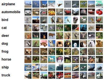
We will look at this tutorial for training a classifier that uses the CIFAR10 dataset. It has the classes: ‘airplane’, ‘automobile’, ‘bird’, ‘cat’, ‘deer’, ‘dog’, ‘frog’, ‘horse’, ‘ship’, ‘truck’. The images in CIFAR-10 are of size 3x32x32, i.e. 3-channel color images of 32x32 pixels in size.

How to train an image classifier

To begin training an image classifier, you have to first load and normalize the CIFAR10 training and test datasets using torchvision. Once you do that, move forth by defining a convolutional neural network. The third step is to define a loss function. Next, train the network on the training data, and lastly, test the network on the test data.

We will now look at each step in details:

1. Loading CIFAR 10 using Torchvision.

**import** torch
**import** torchvision
**import** torchvision.transforms **as** transforms

The output of torchvision datasets are PILImage images of range [0, 1]. We transform them to Tensors of normalized range [-1, 1]. .. note:

If running on Windows and you get a BrokenPipeError, try setting the num_worker of torch.utils.data.DataLoader() to 0.

transform **=** transforms**.**Compose([transforms**.**ToTensor(),transforms**.**Normalize((0.5, 0.5, 0.5), (0.5, 0.5, 0.5))])

trainset = torchvision.datasets.CIFAR10(root='./data', train=True, download=True, transform=transform)
trainloader = torch.utils.data.DataLoader(trainset, batch_size=4,shuffle=True, num_workers=2)

testset = torchvision.datasets.CIFAR10(root='./data', train=False,download=True, transform=transform)

testloader = torch.utils.data.DataLoader(testset, batch_size=4, shuffle=False, num_workers=2)

classes = ('plane', 'car', 'bird', 'cat', 'deer', 'dog', 'frog', 'horse', 'ship', 'truck')

Out:

Downloading https://www.cs.toronto.edu/~kriz/cifar-10-python.tar.gz to ./data/cifar-10-python.tar.gz

Extracting ./data/cifar-10-python.tar.gz to ./data

Files already downloaded and verified

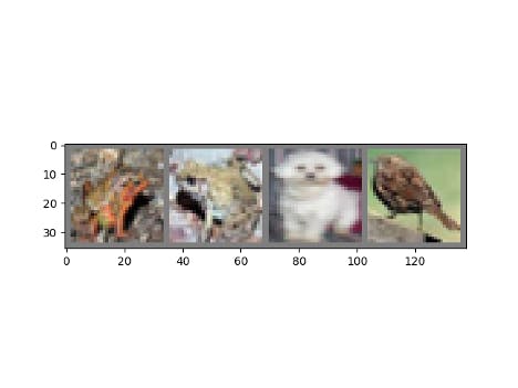
Let’s check out the images.

import matplotlib.pyplot as plt
import numpy as np

# image show
def imshow(img):
   img = img / 2 + 0.5     # unnormalize
   npimg = img.numpy()
   plt.imshow(np.transpose(npimg, (1, 2, 0)))
   plt.show()

# select random images
dataiter = iter(trainloader)
images, labels = dataiter.next()

# show 
imshow(torchvision.utils.make_grid(images))

# show labels
print(' '.join('%5s' % classes[labels[j]] for j in range(4)))

Out

Out:

frog frog dog bird

2. Defining a CNN

Now, you have to copy the neural network from the Neural Networks section before and modify it to take 3-channel images.

import torch.nn as nn
import torch.nn.functional as F

class Net(nn.Module):
    def __init__(self):
        super(Net, self).__init__()
        self.conv1 = nn.Conv2d(3, 6, 5)
        self.pool = nn.MaxPool2d(2, 2)
        self.conv2 = nn.Conv2d(6, 16, 5)
        self.fc1 = nn.Linear(16 * 5 * 5, 120)
        self.fc2 = nn.Linear(120, 84)
        self.fc3 = nn.Linear(84, 10)

def forward(self, x):
        x = self.pool(F.relu(self.conv1(x)))
        x = self.pool(F.relu(self.conv2(x)))
        x = x.view(-1, 16 * 5 * 5)
        x = F.relu(self.fc1(x))
        x = F.relu(self.fc2(x))
        x = self.fc3(x)
        return x

net = Net()

3. Define a Loss function and optimizer

For this, you can use a classification cross-entropy loss and SGD with momentum.

**import** torch.optim **as** optim

criterion = nn.CrossEntropyLoss()

optimizer = optim.SGD(net.parameters(), lr=0.001, momentum=0.9)

4. Training the neural network

A crucial and interesting step in training the classifier; you simply have to loop over the data iterator and feed the inputs to the network and optimize.

for epoch in range(2):  # loop over the dataset multiple times
    running_loss = 0.0
    for i, data in enumerate(trainloader, 0):
        # get the inputs; data is a list of [inputs, labels]
        inputs, labels = data

# zero the parameter gradients
        optimizer.zero_grad()

# forward + backward + optimize
        outputs = net(inputs)
        loss = criterion(outputs, labels)
        loss.backward()
        optimizer.step()

# print statistics
        running_loss += loss.item()
        if i % 2000 == 1999:    # print every 2000 mini-batches
            print('[%d, %5d] loss: %.3f' %
                  (epoch + 1, i + 1, running_loss / 2000))
            running_loss = 0.0

print('Finished Training')

# print statistics
        running_loss += loss.item()
        if i % 2000 == 1999:    # print every 2000 mini-batches
            print('[%d, %5d] loss: %.3f' %
                  (epoch + 1, i + 1, running_loss / 2000))
            running_loss = 0.0

print('Finished Training')

At this stage, don’t forget to save your trained model:

PATH **=** './cifar_net.pth'

torch.save(net.state_dict(), PATH)

You can also follow this guide to learn more about saving Pytorch models correctly.

5. Test the neural network on the test dataset

Now that the training is complete, it is time to test the network. To check if the network has learnt anything, we will predict the class label that the neural network outputs, and check it against the ground-truth.

If the prediction is correct, we add the sample to the list of correct predictions.

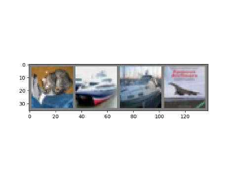
The first step here will require you to display an image from the test set to get familiar.

dataiter = iter(testloader)
images, labels = dataiter.next()

# print images
imshow(torchvision.utils.make_grid(images))
print('GroundTruth: ', ' '.join('%5s' % classes[labels[j]] for j in range(4)))

Output

Out:
GroundTruth:    cat  ship  ship plane

Now, load back in the saved model.

net **=** Net()

net.load_state_dict(torch.load(PATH))

You can now check what this neural network thinks these examples above are:

outputs **=** net(images)

The outputs are energies for the 10 classes. The higher the energy for a class, the more the network thinks that the image is of the particular class. So, let’s get the index of the highest energy:

_, predicted **=** torch**.**max(outputs, 1)
print('Predicted: ', ' '**.**join('%5s' **%** classes[predicted[j]] **for** j **in** range(4)))

Out:

Predicted:    cat  ship plane plane

The results seem pretty good.

Let us look at how the network performs on the whole dataset

correct = 0
total = 0
with torch.no_grad():
    for data in testloader:
        images, labels = data
        outputs = net(images)
        _, predicted = torch.max(outputs.data, 1)
        total += labels.size(0)
        correct += (predicted == labels).sum().item()

print('Accuracy of the network on the 10000 test images: %d %%' % (
    100 * correct / total))

Out:
Accuracy of the network on the 10000 test images: 57 %

That looks way better than chance, which is 10% accuracy (randomly picking a class out of 10 classes). This shows that the network has learnt something.

Now, let’s look at the classes that performed well and the classes that did not perform well:

class_correct = list(0. for i in range(10))
class_total = list(0. for i in range(10))
with torch.no_grad():
    for data in testloader:
        images, labels = data
        outputs = net(images)
        _, predicted = torch.max(outputs, 1)
        c = (predicted == labels).squeeze()
        for i in range(4):
            label = labels[i]
            class_correct[label] += c[i].item()
            class_total[label] += 1

for i in range(10):
    print('Accuracy of %5s : %2d %%' % (
        classes[i], 100 * class_correct[i] / class_total[i]))

Out:
Accuracy of plane : 63 %
Accuracy of   car : 59 %
Accuracy of  bird : 37 %
Accuracy of   cat : 24 %
Accuracy of  deer : 53 %
Accuracy of   dog : 64 %
Accuracy of  frog : 73 %
Accuracy of horse : 62 %
Accuracy of  ship : 65 %
Accuracy of truck : 72 %

Next, we can run these neural networks on the GPU.

Training on GPU

Similar to how you would transfer a Tensor onto the GPU, you will transfer the neural net onto the GPU. First, we need to define the device as the first visible cuda device if we have CUDA available:

device **=** torch**.**device("cuda:0" **if** torch**.**cuda**.**is_available() **else **"cpu")
*# Assuming that we are on a CUDA machine, this should print a CUDA device:
*print(device)
Out:
Cuda:0

The rest of this section assumes that the device is a CUDA device.

Then these methods will recursively go over all modules and convert their parameters and buffers to CUDA tensors:

net**.**to(device)

Remember that you will have to send the inputs and targets at every step to the GPU too:

inputs, labels **=** data[0]**.**to(device), data[1]**.**to(device)

You may notice that there is no massive speedup compared to CPU, this is because your network is small. To address this, try increasing the width of your network (argument 2 of the first nn.Conv2d, and argument 1 of the second nn.Conv2d — they need to be the same number), and see what kind of speedup you get.

Conclusion

By following the tutorial above, you have successfully managed to train a small neural network to classify images.

Looking for more details?

Checkout this video on my YouTube Channel

Follow Me on Linkedin & Twitter

If you are interested in similar content do follow me on Twitter and Linkedin

Linkedin: https://www.linkedin.com/in/anuj-syal-727736101/

Twitter: https://twitter.com/anuj_syal