Photo by Genessa Panainte on Unsplash

Machine learning that is applied to build personalizations, suggestions, and future analyses are becoming increasingly important as companies generate increasingly diversified and user-focused digital goods and solutions. Rather than dealing with the complications of different datasets, the Apache Spark machine learning library (MLlib) enables data engineers to concentrate on specific data challenges and algorithms.

A linear technique to modeling the connection across a dependent factor and one or maybe more random factors is known as linear regression. It is one of the most fundamental and widely used kinds of predictive modeling.

What is Spark MLlib?

Photo by Marius Masalar on Unsplash

Spark MLlib is among the most appealing features of Spark as it has the capacity to enormously scale processing, which is precisely what machine learning models require. However, there are some machine learning models that cannot be properly implemented, which is a drawback.

MLlib is a comprehensive machine learning package that includes categorization, regression, clustering, cooperative filtration, and fundamental optimal primitives, as well as other popular learning methods and tools.

##What is linear regression model?

By matching a line to the given information, regression methods illustrate the connection among variables. A straight line is used in this system, whereas a curved path is used in nonlinear systems.

You can also start using regression to predict the characteristics of a dependent variable that depends on the characteristics of an independent variable. The link among two qualitative parameters is estimated using simple linear regression.

Why to use spark Mllib for ml

Spark is a strong, centralized platform for data scientists due to its fast speed. It is also a simple to use tool that helps them get desired results quickly. This enables data scientists to fix deep learning complications along with pattern calculation, broadcasting, and interactive request handling at a much larger scale.

R, Python and Java, are just a few of the languages available in Spark. The 2015 Spark Study, which interviewed the Spark community, revealed that Python and R have seen primarily fast growth. In particular, 58 percent of participants said they used Python and 18 percent said they were currently utilising the R API.

Interested in more comprehensive tutorial:

Check out this youtube video:

Create your first linear regression model with Spark Mllib

• Step 1: Pyspark environment setup For pyspark environment on local machine, my preferred option is to use docker to run jupyter/pyspark-notebook image. However, if you are interested in an extensive installation guide check out my blog post or youtube video

• Step 2: Create a spark session

from pyspark.sql import SparkSession
spark = SparkSession.builder.master("local").appName("linear_regression_model").getOrCreate()

• Step3: Load dataset

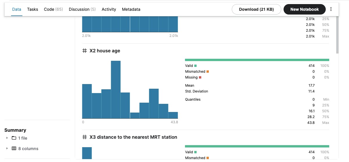
For the dataset, I am using a simple Real Estate dataset from Kaggle , which contains a simple data for real estate with continuous features like distance from mrt station, coordinates, size, etc

After you download read the dataset into a spark dataframe

real_estate = spark.read.option("inferSchema", "true").csv("real_estate.csv",header=True)

• Step4: Explore data and its attribute

We can explore different attributes/columns of the data using a few inbuilt functions in spark.

PrintSchema() to see the columns with data types

real_estate.printSchema()
Out:
root
 |-- No: integer (nullable = true)
 |-- X1 transaction date: double (nullable = true)
 |-- X2 house age: double (nullable = true)
 |-- X3 distance to the nearest MRT station: double (nullable = true)
 |-- X4 number of convenience stores: integer (nullable = true)
 |-- X5 latitude: double (nullable = true)
 |-- X6 longitude: double (nullable = true)
 |-- Y house price of unit area: double (nullable = true)

Show() Check out a few rows and understand the data

real_estate.show(2)
Out:
+---+-------------------+------------+--------------------------------------+-------------------------------+-----------+------------+--------------------------+
| No|X1 transaction date|X2 house age|X3 distance to the nearest MRT station|X4 number of convenience stores|X5 latitude|X6 longitude|Y house price of unit area|
+---+-------------------+------------+--------------------------------------+-------------------------------+-----------+------------+--------------------------+
|  1|           2012.917|        32.0|                              84.87882|                             10|   24.98298|   121.54024|                      37.9|
|  2|           2012.917|        19.5|                              306.5947|                              9|   24.98034|   121.53951|                      42.2|
+---+-------------------+------------+--------------------------------------+-------------------------------+-----------+------------+--------------------------+
only showing top 2 rows

describe() to see statistics of columns

real_estate.describe().show()
Out:
+-------+-----------------+-------------------+------------------+--------------------------------------+-------------------------------+--------------------+--------------------+--------------------------+
|summary|               No|X1 transaction date|      X2 house age|X3 distance to the nearest MRT station|X4 number of convenience stores|         X5 latitude|        X6 longitude|Y house price of unit area|
+-------+-----------------+-------------------+------------------+--------------------------------------+-------------------------------+--------------------+--------------------+--------------------------+
|  count|              414|                414|               414|                                   414|                            414|                 414|                 414|                       414|
|   mean|            207.5| 2013.1489710144933| 17.71256038647343|                    1083.8856889130436|              4.094202898550725|  24.969030072463745|  121.53336108695667|         37.98019323671498|
| stddev|119.6557562342907| 0.2819672402629999|11.392484533242524|                     1262.109595407851|             2.9455618056636177|0.012410196590450208|0.015347183004592374|        13.606487697735316|
|    min|                1|           2012.667|               0.0|                              23.38284|                              0|            24.93207|           121.47353|                       7.6|
|    max|              414|           2013.583|              43.8|                              6488.021|                             10|            25.01459|           121.56627|                     117.5|
+-------+-----------------+-------------------+------------------+--------------------------------------+-------------------------------+--------------------+--------------------+--------------------------+

Kaggle also provides the details on these attributes such as count, mean, standard deviation. This will allow you to decide on which parameters to use as features for the model

• Step4: VectorAssembler to transform data into feature columns

After you have decided which columns to use VectorAssembler to format the dataframe

from pyspark.ml.feature import VectorAssembler

assembler = VectorAssembler(inputCols=[ 
 'X1 transaction date',
 'X2 house age',
 'X3 distance to the nearest MRT station',
 'X4 number of convenience stores',
 'X5 latitude',
 'X6 longitude'],
 outputCol='features')

data_set = assembler.transform(real_estate)
data_set.select(['features','Y house price of unit area']).show(2)

Out:
+--------------------+--------------------------+
|            features|Y house price of unit area|
+--------------------+--------------------------+
|[2012.917,32.0,84...|                      37.9|
|[2012.917,19.5,30...|                      42.2|
+--------------------+--------------------------+
only showing top 2 rows

• Step5: Split into Train and Test set

train_data,test_data = final_data.randomSplit([0.7,0.3])

• Step 6: Train your model (Fit your model with train data)

from pyspark.ml.regression import LinearRegression

lr = LinearRegression(labelCol='Y house price of unit area')
lrModel = lr.fit(train_data)

• Step6: Perform descriptive analysis with correlation

Check out coefficients after validating with the test set:

test_stats = lrModel.evaluate(test_data)
print(f"RMSE: {test_stats.rootMeanSquaredError}")
print(f"R2: {test_stats.r2}")
print(f"R2: {test_stats.meanSquaredError}")

Out:
RMSE: 7.553238336636628
R2: 0.6493363975473592
R2: 57.051409370037256

Root Mean Squared Error (RMSE) on test data = 7.553238336636628

Conclusion

Spark isn't just a better approach to comprehend our information; it's also a lot faster. Spark transforms data analytics and research by enabling us to handle a wide variety of data challenges in a preferred language. Spark MLlib makes it simple for new data scientists to engage with their models right out of the package and specialists can fine-tune as needed.

Distributed networks could be the subject of data engineers, while machine learning methods and algorithms might be the subject of data scientists. Spark has significantly improved and revolutionized the machine learning by allowing data scientists to concentrate on the data challenges that matter to them while openly utilizing Spark's single system's performance, convenience, and integration.